noisyR count matrix approach workflow
Source:vignettes/vignette_noisyr_counts.Rmd
vignette_noisyr_counts.RmdThe noisyR package is an end-to-end pipeline for quantifying and removing technical noise from HTS datasets. The three main pipeline steps are:
- similarity calculation
- noise quantification
- noise removal
Each step can be finely tuned using hyperparameters; optimal, data-driven values for these parameters are also determined.
The package and some applications are described in more detail in this publication and is actively maintained on https://github.com/Core-Bioinformatics/noisyR.
The count matrix approach uses the original, un-normalised count matrix, as provided after alignment and feature quantification; each sample is processed individually, only the relative expressions across samples are compared. Relying on the hypothesis that the majority of genes are not DE, most of the evaluations are expected to point towards a high similarity across samples.
Installation
To install the package, first install all bioconductor dependencies:
packages.bioc <- c("preprocessCore",
                   "IRanges",
                   "GenomicRanges",
                   "Rsamtools")
new.packages.bioc <- packages.bioc[!(packages.bioc %in% installed.packages()[,"Package"])]
if(length(new.packages.bioc)){
  if (!requireNamespace("BiocManager", quietly = TRUE))
    install.packages("BiocManager")
  BiocManager::install(new.packages.bioc)
}
Then, you can install noisyR (and all its other dependencies) from CRAN:
install.packages("noisyr")To install the latest stable version from GitHub, first install CRAN dependencies:
packages.cran <- c("utils",
                   "grDevices",
                   "tibble",
                   "dplyr",
                   "magrittr",
                   "ggplot2",
                   "philentropy",
                   "doParallel",
                   "foreach")
new.packages.cran <- packages.cran[!(packages.cran %in% installed.packages()[,"Package"])]
if(length(new.packages.cran))
  install.packages(new.packages.cran)

if (!requireNamespace("devtools", quietly = TRUE))
  install.packages("devtools")
devtools::install_github("Core-Bioinformatics/noisyR")
Preprocessing
First, load noisyR:
library(noisyr)
#> Welcome to noisyr!
#> Have a look at our website to get started:
#>   https://core-bioinformatics.github.io/noisyR/
#> To cite noisyr in publications please use:
#>   10.1093/nar/gkab433
For this demonstration we will be using a subset of the count matrix for an experiment included in a 2019 paper by Yang et al. Rows represent genes/features and columns represent samples:
counts.in <- system.file("extdata", "counts_raw.csv", package = "noisyr")
df <- read.csv(counts.in, row.names = 1)
str(df)
#> 'data.frame':    55573 obs. of  4 variables:
#>  $ SRR7624365: int  2 0 6 0 0 0 0 0 0 0 ...
#>  $ SRR7624366: int  0 0 4 0 0 0 0 0 0 0 ...
#>  $ SRR7624371: int  0 0 2 0 2 0 0 0 0 0 ...
#>  $ SRR7624372: int  0 0 0 0 0 2 0 0 0 0 ...
head(df)
#>                    SRR7624365 SRR7624366 SRR7624371 SRR7624372
#> ENSMUSG00000102693          2          0          0          0
#> ENSMUSG00000064842          0          0          0          0
#> ENSMUSG00000051951          6          4          2          0
#> ENSMUSG00000102851          0          0          0          0
#> ENSMUSG00000103377          0          0          2          0
#> ENSMUSG00000104017          0          0          0          2
Note that when reading from a file R typically returns a data frame. To convert to a matrix we use the function cast_matrix_to_numeric(). This also converts values to numeric (in case they were read as characters). Any values that are not coercible to numeric are replaced by 0.
expression.matrix <- noisyr::cast_matrix_to_numeric(df)Running noisyR
The full noisyR pipeline can be run through noisyr(), choosing “counts” for the count matrix approach (internally calls noisyr_counts()). The user can pass many arguments to this function, which alter the behaviour of the different pipeline steps, as discussed in the breakdown below.
expression.matrix.denoised.standard <- noisyr::noisyr(
  approach.for.similarity.calculation = "counts",
  expression.matrix = df
)
#> >>> noisyR counts approach pipeline <<<
#> The input matrix has 55573 rows and 4 cols
#>     number of genes: 55573
#>     number of samples: 4
#> Calculating the number of elements per window
#>     the number of elements per window is 5557
#>     the step size is 277
#>     the selected similarity metric is correlation_pearson
#>   Working with sample 1
#>   Working with sample 2
#>   Working with sample 3
#>   Working with sample 4
#> Calculating noise thresholds for 4 samples...
#>     similarity.threshold = 0.25
#>     method.chosen = Boxplot-IQR
#> Denoising expression matrix...
#>     removing noisy genes
#>     adjusting matrix
#> >>> Done! <<<
The output of the noise removal is a denoised matrix that can be passed on to other methods for downstream analysis.
head(expression.matrix.denoised.standard)
#>                    SRR7624365 SRR7624366 SRR7624371 SRR7624372
#> ENSMUSG00000025902         94         74         32         44
#> ENSMUSG00000102269         24         48         20         26
#> ENSMUSG00000098104         76         68         62         60
#> ENSMUSG00000103922        326        273        318        365
#> ENSMUSG00000033845      14451       9925      14702      14549
#> ENSMUSG00000102275        117        100        142        124
apply(expression.matrix.denoised.standard, 2, min)
#> SRR7624365 SRR7624366 SRR7624371 SRR7624372
#>         18         18         18         18
Pipeline breakdown
While for most applications, running noisyr() is sufficient, it may be useful to run individual pipeline steps manually. For example, the user may want to create summary figures for the denoising, store the noise thresholds obtained or other intermediary outputs, or try out different options without rerunning all steps. In this section, we look deeper into noisyr() and break down the three main steps that are performed.
Similarity calculation
We can then run the similarity calculation using calculate_expression_similarity_counts():
expression.summary <- noisyr::calculate_expression_similarity_counts(
  expression.matrix = expression.matrix,
  similarity.measure = "correlation_pearson"
)
#> The input matrix has 55573 rows and 4 cols
#>     number of genes: 55573
#>     number of samples: 4
#> Calculating the number of elements per window
#>     the number of elements per window is 5557
#>     the step size is 277
#>     the selected similarity metric is correlation_pearson
#>   Working with sample 1
#>   Working with sample 2
#>   Working with sample 3
#>   Working with sample 4
str(expression.summary)
#> List of 3
#>  $ expression.matrix           : num [1:55573, 1:4] 2 0 6 0 0 0 0 0 0 0 ...
#>   ..- attr(*, "dimnames")=List of 2
#>   .. ..$ : chr [1:55573] "ENSMUSG00000102693" "ENSMUSG00000064842" "ENSMUSG00000051951" "ENSMUSG00000102851" ...
#>   .. ..$ : chr [1:4] "SRR7624365" "SRR7624366" "SRR7624371" "SRR7624372"
#>  $ expression.levels           : num [1:181, 1:4] 0 0 0 0 0 0 0 0 0 0 ...
#>  $ expression.levels.similarity: num [1:181, 1:4] NA NA NA NA NA NA NA NA NA NA ...
Users can select a similarity measure to assess the localised consistency in expression across samples (dissimilarity measures are inverted). See the philentropy package documentation for more information on the different distances. The full list of available metrics can be viewed by:
noisyr::get_methods_correlation_distance()
#>  [1] "correlation_pearson"        "correlation_kendall"
#>  [3] "correlation_spearman"       "distance_euclidean"
#>  [5] "distance_manhattan"         "distance_minkowski"
#>  [7] "distance_chebyshev"         "distance_sorensen"
#>  [9] "distance_gower"             "distance_soergel"
#> [11] "distance_kulczynski_d"      "distance_canberra"
#> [13] "distance_lorentzian"        "distance_intersection"
#> [15] "distance_non-intersection"  "distance_wavehedges"
#> [17] "distance_czekanowski"       "distance_motyka"
#> [19] "distance_kulczynski_s"      "distance_tanimoto"
#> [21] "distance_ruzicka"           "distance_inner_product"
#> [23] "distance_harmonic_mean"     "distance_cosine"
#> [25] "distance_hassebrook"        "distance_jaccard"
#> [27] "distance_dice"              "distance_fidelity"
#> [29] "distance_bhattacharyya"     "distance_hellinger"
#> [31] "distance_matusita"          "distance_squared_chord"
#> [33] "distance_squared_euclidean" "distance_pearson"
#> [35] "distance_neyman"            "distance_squared_chi"
#> [37] "distance_prob_symm"         "distance_divergence"
#> [39] "distance_clark"             "distance_additive_symm"
#> [41] "distance_kullback-leibler"  "distance_jeffreys"
#> [43] "distance_k_divergence"      "distance_topsoe"
#> [45] "distance_jensen-shannon"    "distance_jensen_difference"
#> [47] "distance_taneja"            "distance_kumar-johnson"
#> [49] "distance_avg"
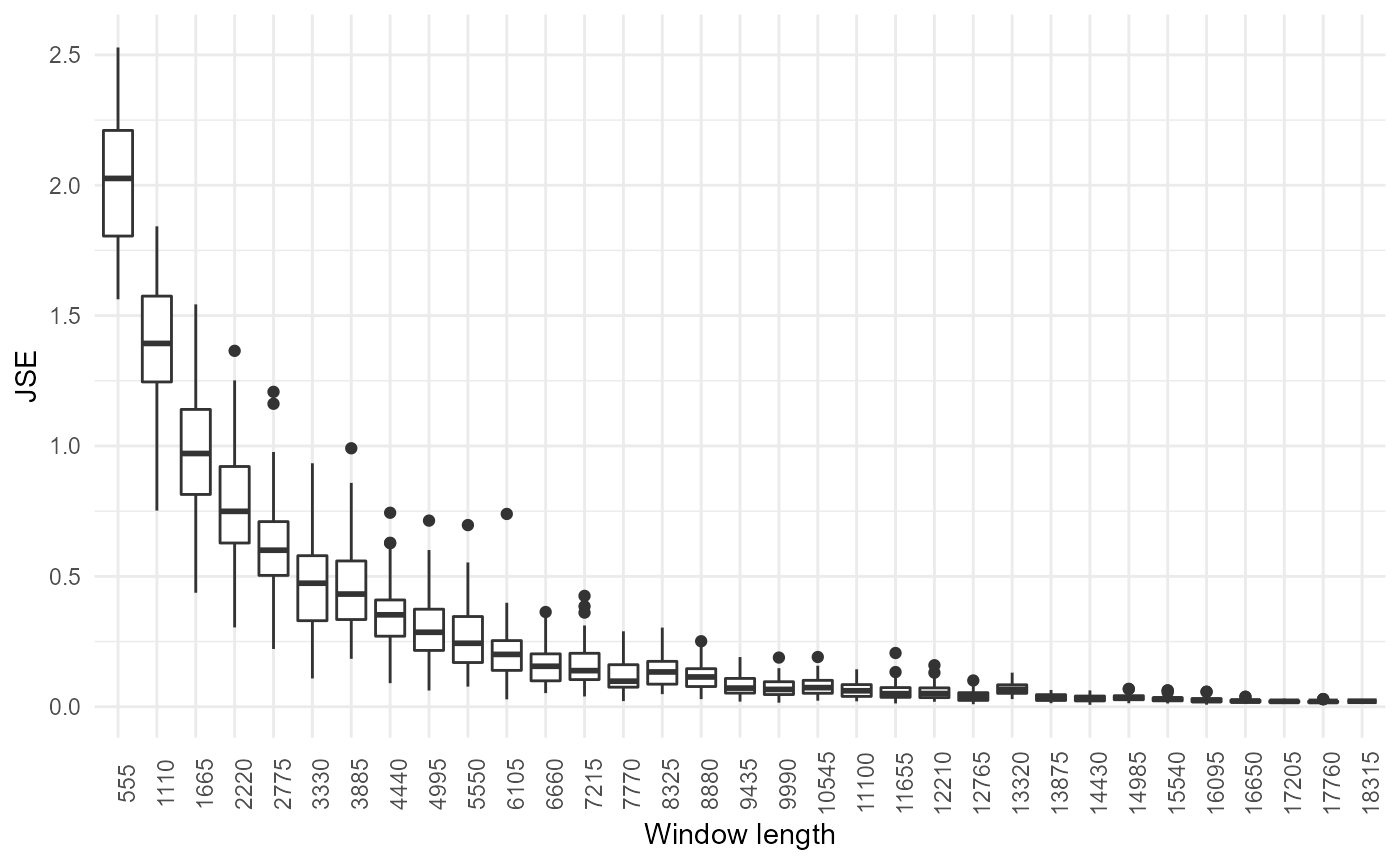
By default, the window length is 10% of the number of rows in the matrix, as it has proven effective empirically. A different window can be specified by the n.elements.per.window parameter. The optimal window length can also be estimated by seeking stability of output (but this can be computationally intensive for large datasets):
noisyr::optimise_window_length(
  expression.matrix = expression.matrix,
  similarity.measure = "correlation_pearson"
)
#> Window length optimisation
#>     number of windows: 33
#>     minimum window: 555
#>     maximum window: 18339
#>     window step: 555
#>     # of iterations: 50
#>     minimum similar windows: 3
#> Calculating expression summary and JSE for each window...
#> Performing t-tests...
#> The number of similar windows found for each window (including itself) were:
#>     1 1 1 1 1 2 2 1 2 2 1 3 3 3 5 3 4 6 4 5 5 3 3 6 5 4 4 4 2 3 4 2 3
#> Optimal window found!
#> [1] 6660Window length optimisation can be turned on using the optimise.window.length.logical parameter in noisyr() or noisyr_counts().
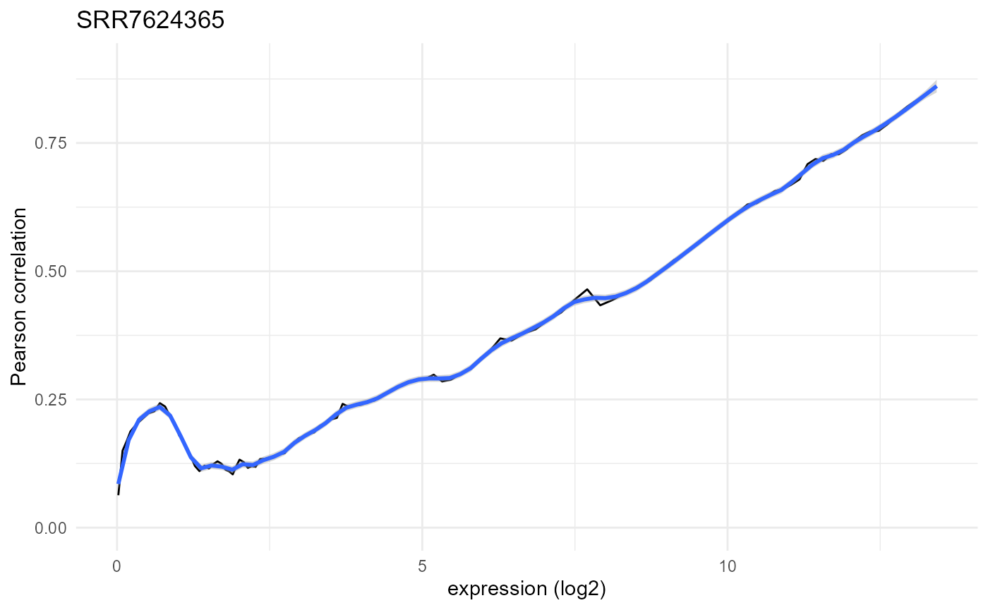
Plots of the abundance-correlation relation can be generated through the plot_expression_similarity() function:
plotlist <- noisyr::plot_expression_similarity(
  expression.summary = expression.summary)
plotlist[[1]]
As expected, we observe low correlation values for low abundances and a steady increase towards 1 as the abundance increases. This is based on the expectation that most genes are not differentially expressed and have consistent expression, but at low abundances the stochastic nature of transcription and sequencing gives rise to noise. The local maximum at very low abundances is due to strings of zeros driving the correlation higher than expected.
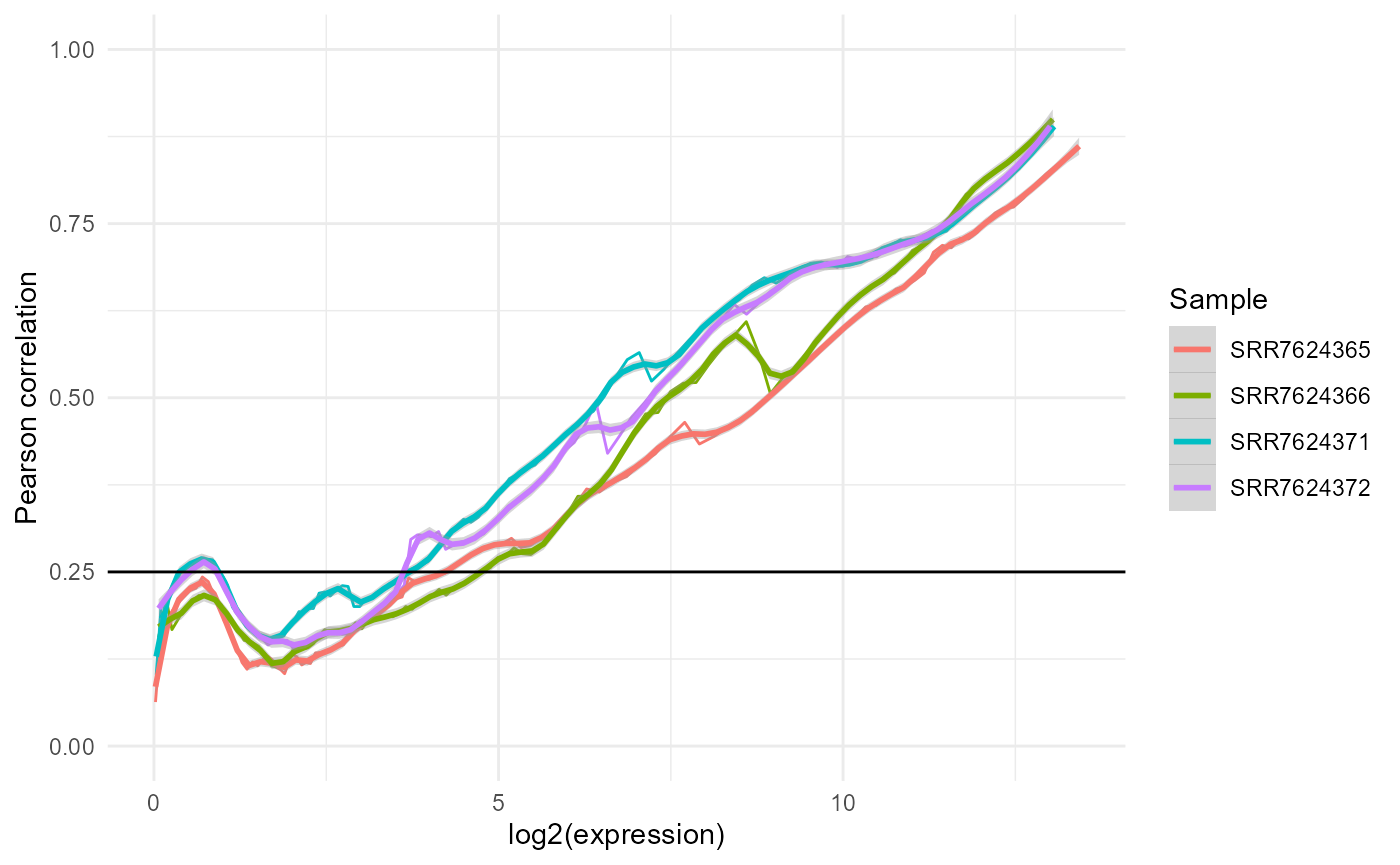
These are ggplot objects, and can thus be modified and combined intuitively. For example, plotting all the line plots together:
plotdf.line <- tibble::tibble()
for(i in 1:4){
  lineid <- i * 2 - 1
  plotdf.line <- rbind(
    plotdf.line,
    dplyr::mutate(plotlist[[lineid]]$data,
                  Sample=colnames(expression.matrix)[i]))
}

ggplot2::ggplot(plotdf.line) +
    ggplot2::theme_minimal() +
    ggplot2::geom_line(ggplot2::aes(x=x, y=y, colour=Sample)) +
    ggplot2::geom_smooth(ggplot2::aes(x,y,colour=Sample), method="loess",
                         formula= y ~ x, span=0.1) +
    ggplot2::ylim(0:1) +
    ggplot2::xlab("log2(expression)") +
    ggplot2::ylab("Pearson correlation") +
    ggplot2::geom_hline(yintercept=0.25, color="black")
Noise quantification
Using the output of the similarity calculation, we can compute the signal to noise threshold in each sample:
noise.thresholds <- noisyr::calculate_noise_threshold(expression = expression.summary)
#> Calculating noise thresholds for 4 samples...
#>     similarity.threshold = 0.25
#>     method.chosen = Boxplot-IQR
noise.thresholds
#> [1] 19.69831 25.99208 12.12573 12.99604
Here we used the default parameters: a similarity threshold of 0.25 and the Boxplot-IQR method. There are several methods available, which can be viewed with the get_methods_calculate_noise_threshold() function:
noisyr::get_methods_calculate_noise_threshold()
#>  [1] "Density_based-No_normalisation"
#>  [2] "Density_based-RPM_normalisation"
#>  [3] "Density_based-Quantile_normalisation"
#>  [4] "Line_plot-No_smoothing"
#>  [5] "Line_plot-loess10_smoothing"
#>  [6] "Line_plot-loess25_smoothing"
#>  [7] "Line_plot-loess50_smoothing"
#>  [8] "Boxplot-Median"
#>  [9] "Boxplot-IQR"
#> [10] "Boxplot-Quant5"
The first three methods are just calculating the minimum of the density plot for all genes (a common, fast approach). This usually provides a rough, overestimated signal to noise threshold.
The rest of the methods use either the (smoothed) line plot or the boxplot to find the noise threshold given a similarity (correlation/distance) threshold.
It is recommended that the method with the least coefficient of variation across all samples is chosen for noise removal. This can also be applied to compute the correlation/distance threshold instead of supplying it manually, which is especially useful for non-correlation measures which don’t have a standard range.
For example, by looking to minimise the coefficient of variation, we get a correlation threshold of 0.21 and the loess10 smoothing method for this dataset (by default all methods from get_methods_calculate_noise_threshold() are used:
similarity.threshold.sequence <- seq(0.2, 0.3, by=0.01)
stats.table <- noisyr::calculate_noise_threshold_method_statistics(
  expression = expression.summary,
  similarity.threshold.sequence = similarity.threshold.sequence
)
row.min.coef.var <- which.min(stats.table$noise.threshold.coefficient.of.variation)
# adjust column names for printing
colnames(stats.table) <- c("approach", "method", "corr.thr", "min", "mean", "coef.var", "max", "all")
stats.table[row.min.coef.var, 1:7]
#> # A tibble: 1 x 7
#>   approach  method            corr.thr   min  mean coef.var   max
#>   <chr>     <chr>                <dbl> <dbl> <dbl>    <dbl> <dbl>
#> 1 Line_plot loess10_smoothing     0.21  7.37  9.88    0.253  13.3
dplyr::filter(stats.table, round(corr.thr, 2) == 0.21)[, 1:7]
#> # A tibble: 10 x 7
#>    approach      method                 corr.thr    min   mean coef.var   max
#>    <chr>         <chr>                     <dbl>  <dbl>  <dbl>    <dbl> <dbl>
#>  1 Density_based No_normalisation           0.21 308    308      NA     308
#>  2 Density_based RPM_normalisation          0.21 290    290      NA     290
#>  3 Density_based Quantile_normalisation     0.21 304    304      NA     304
#>  4 Line_plot     No_smoothing               0.21   0      0     NaN       0
#>  5 Line_plot     loess10_smoothing          0.21   7.37   9.88    0.253  13.3
#>  6 Line_plot     loess25_smoothing          0.21   4.26   9.20    0.450  14.3
#>  7 Line_plot     loess50_smoothing          0.21   6.47   9.92    0.336  14.3
#>  8 Boxplot       Median                     0.21   8.57  11.6     0.271  16
#>  9 Boxplot       IQR                        0.21   8.57  11.6     0.271  16
#> 10 Boxplot       Quant5                     0.21   8.57  11.6     0.271  16
dplyr::filter(stats.table, method == "loess10_smoothing")[, 1:7]
#> # A tibble: 11 x 7
#>    approach  method            corr.thr   min  mean coef.var   max
#>    <chr>     <chr>                <dbl> <dbl> <dbl>    <dbl> <dbl>
#>  1 Line_plot loess10_smoothing     0.2   3.72  8.42    0.425  12.4
#>  2 Line_plot loess10_smoothing     0.21  7.37  9.88    0.253  13.3
#>  3 Line_plot loess10_smoothing     0.22  8.42 11.3     0.321  16.6
#>  4 Line_plot loess10_smoothing     0.23  9.02 12.7     0.358  19.3
#>  5 Line_plot loess10_smoothing     0.24 10.4  14.3     0.395  22.5
#>  6 Line_plot loess10_smoothing     0.25 10.6  16.1     0.388  24.3
#>  7 Line_plot loess10_smoothing     0.26 11.4  17.9     0.433  28.4
#>  8 Line_plot loess10_smoothing     0.27 11.4  19.4     0.439  30.8
#>  9 Line_plot loess10_smoothing     0.28 12.2  24.0     0.578  43.3
#> 10 Line_plot loess10_smoothing     0.29 15.9  28.0     0.505  47.4
#> 11 Line_plot loess10_smoothing     0.3  17.1  35.4     0.486  52.0
We can then call calculate_noise_threshold() with our optimised parameters:
noise.thresholds <- noisyr::calculate_noise_threshold(
  expression = expression.summary,
  similarity.threshold = 0.21,
  method.chosen = "Line_plot-loess10_smoothing"
)
#> Calculating noise thresholds for 4 samples...
#>     similarity.threshold = 0.21
#>     method.chosen = Line_plot-loess10_smoothing
noise.thresholds
#> [1]  9.664027 13.325175  7.368364  9.171495
Parameter optimisation can be turned on by specifying vectors of values for similarity.threshold and/or method.chosen (a subset of get_methods_calculate_noise_threshold()) when calling noisyr() or noisyr_counts().
Noise removal
To produce the denoised count matrix, the function remove_noise_from_matrix() is used with a specified vector of noise thresholds (usually calculated by calculate_noise_threshold()).
expression.matrix.denoised <- noisyr::remove_noise_from_matrix(
  expression.matrix = expression.matrix,
  noise.thresholds = noise.thresholds)
#> Denoising expression matrix...
#>     removing noisy genes
#>     adjusting matrix
str(expression.matrix.denoised)
#>  num [1:24341, 1:4] 17 86 16 68 318 ...
#>  - attr(*, "dimnames")=List of 2
#>   ..$ : chr [1:24341] "ENSMUSG00000102343" "ENSMUSG00000025902" "ENSMUSG00000102269" "ENSMUSG00000098104" ...
#>   ..$ : chr [1:4] "SRR7624365" "SRR7624366" "SRR7624371" "SRR7624372"
The behaviour of remove_noise_from_matrix() can be further modified:
- add.threshold whether to add the noise threshold to each entry (default) or set each entry under the noise threshold to the noise threshold.
-
average.threshold whether the noise thresholds for the different samples are averaged (default) or used individually. The latter should be especially avoided if the thresholds have high variance, as it could intoduce artificial differences in the data.
- remove.noisy.features whether genes/features whose expression is under the noise threshold in every sample should be removed from the matrix (default) or not
Because of these defaults, passing the mean of the thresholds gives a slightly different result (different # of genes fully under the noise threshold:
expression.matrix.denoised.fixed <- noisyr::remove_noise_from_matrix(
  expression.matrix = expression.matrix,
  noise.thresholds = mean(noise.thresholds))
#> noise.thresholds only has 1 value, using a fixed threshold...
#> Denoising expression matrix...
#>     removing noisy genes
#>     adjusting matrix
nrow(expression.matrix.denoised); nrow(expression.matrix.denoised.fixed)
#> [1] 24341
#> [1] 24309
By supplying the corresponding parameters to noisyr(), we obtain the same final result from the full pipeline:
expression.matrix.denoised.full.pipeline <- noisyr::noisyr(
  approach.for.similarity.calculation = "counts",
  expression.matrix = expression.matrix,
  similarity.measure = "correlation_pearson",
  optimise.window.length.logical = FALSE,
  similarity.threshold = seq(0.2, 0.3, by=0.01),
  method.chosen = get_methods_calculate_noise_threshold()
)
#> >>> noisyR counts approach pipeline <<<
#> The input matrix has 55573 rows and 4 cols
#>     number of genes: 55573
#>     number of samples: 4
#> Calculating the number of elements per window
#>     the number of elements per window is 5557
#>     the step size is 277
#>     the selected similarity metric is correlation_pearson
#>   Working with sample 1
#>   Working with sample 2
#>   Working with sample 3
#>   Working with sample 4
#> Selecting parameters that minimise the coefficient of variation...
#> Calculating noise thresholds for 4 samples...
#>     similarity.threshold = 0.21
#>     method.chosen = Line_plot-loess10_smoothing
#> Denoising expression matrix...
#>     removing noisy genes
#>     adjusting matrix
#> >>> Done! <<<
identical(expression.matrix.denoised,
          expression.matrix.denoised.full.pipeline)
#> [1] TRUE
Downstream analysis
The denoised matrix can be used instead of the raw count matrix for downstream analysis. Here we present a simple example of a differential expression (DE) analysis and compare the two.
We create a function to perform the same DE pipeline on both matrices, using the edgeR package.
DE_edgeR = function(expression.matrix, metadata){
  # load or install edgeR
  if(!require(edgeR)){
    if (!requireNamespace("BiocManager", quietly = TRUE))
      install.packages("BiocManager")
    BiocManager::install("edgeR")
  }

  # create metadata
  metadata <- data.frame(id = colnames(expression.matrix),
                         timepoint = c("0h", "0h", "12h", "12h"))

  # quantile normalise
  expression.matrix.normalised <-
    preprocessCore::normalize.quantiles(expression.matrix)
  rownames(expression.matrix.normalised) <- base::rownames(expression.matrix)
  colnames(expression.matrix.normalised) <- base::colnames(expression.matrix)

  # process using edgeR
  expression.matrix.for.de <- round(expression.matrix.normalised)
  expression.matrix.for.de <-
    expression.matrix.for.de[apply(expression.matrix.for.de, 1, sum) > 0, ]
  design <- model.matrix(~ 0 + metadata$timepoint)
  edger <- DGEList(counts = expression.matrix.for.de)
  edger <- estimateDisp(edger, design)
  edger.fit <- glmFit(edger, design)
  edger.lrt <- glmLRT(edger.fit, contrast=c(-1, 1))

  # extract results
  res <- topTags(edger.lrt, n = Inf)$table
  res$DE <- res$FDR < 0.05 & abs(res$logFC) > 1

  # make volcano plot
  print(
    ggplot2::ggplot(res) +
      ggplot2::theme_minimal() +
      ggplot2::geom_point(ggplot2::aes(x=logFC,
                                       y=-log10(FDR),
                                       colour=DE),
                          show.legend=FALSE) +
      ggplot2::scale_color_manual(values=c("black", "red")) +
      ggplot2::lims(x=c(-12, 12), y=c(0, 120))
  )

  return(res)

}

results.raw <- DE_edgeR(expression.matrix)
results.denoised <- DE_edgeR(expression.matrix.denoised)
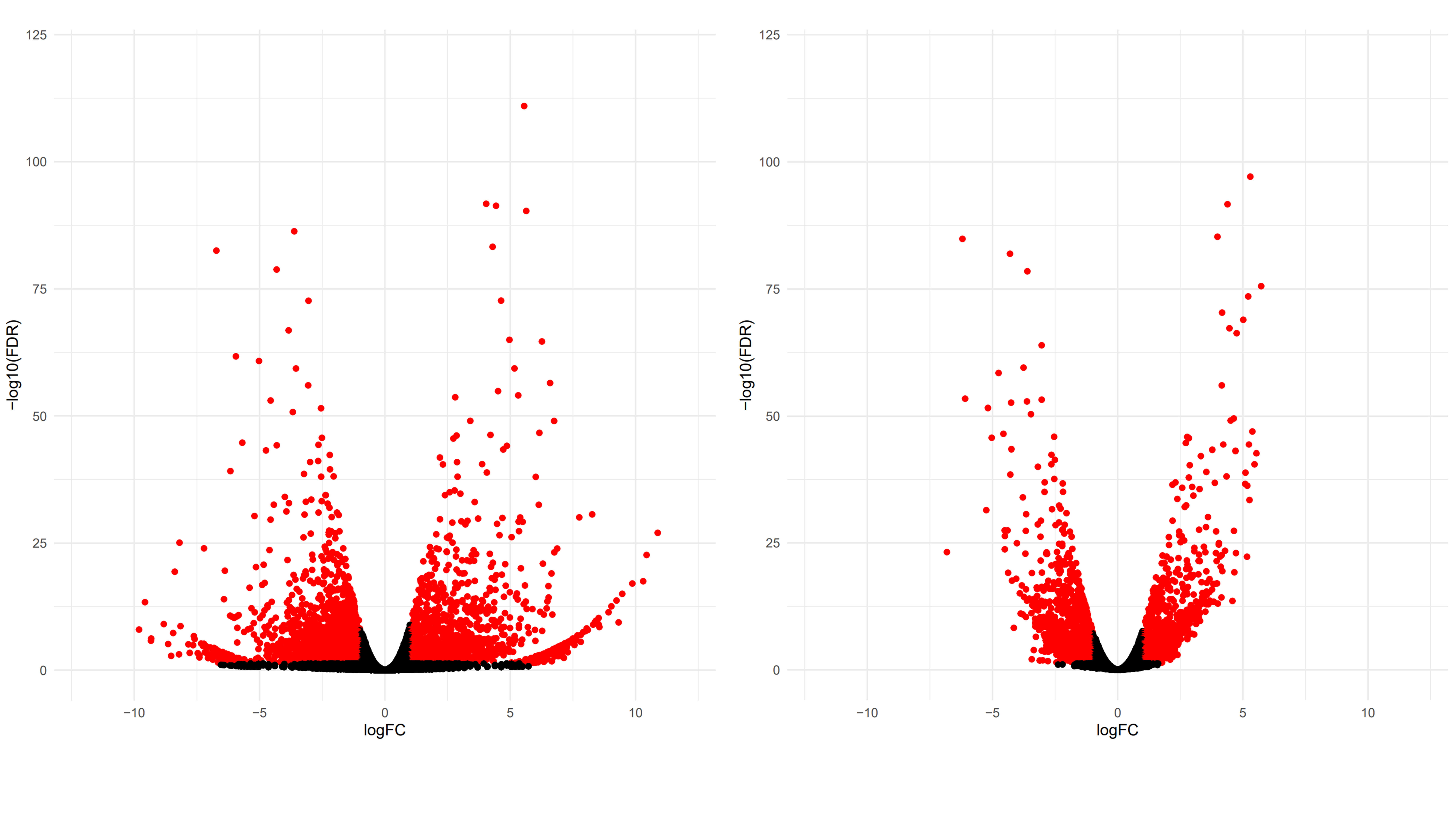
We observe the distribution of genes in the volcano plots becoming a lot tighter for the denoised matrix. For the raw matrix, there are a lot of genes with low p-values and high log-fold changes that are barely called DE. Those “whiskers” are corrected for the denoised matrix.
We can also see the number of differentially expressed genes has been reduced.
sessionInfo()
#> R version 4.1.0 (2021-05-18)
#> Platform: x86_64-w64-mingw32/x64 (64-bit)
#> Running under: Windows 10 x64 (build 19042)
#>
#> Matrix products: default
#>
#> locale:
#> [1] LC_COLLATE=English_United Kingdom.1252
#> [2] LC_CTYPE=English_United Kingdom.1252
#> [3] LC_MONETARY=English_United Kingdom.1252
#> [4] LC_NUMERIC=C
#> [5] LC_TIME=English_United Kingdom.1252
#>
#> attached base packages:
#> [1] stats     graphics  grDevices utils     datasets  methods   base
#>
#> other attached packages:
#> [1] noisyr_1.0.0
#>
#> loaded via a namespace (and not attached):
#>  [1] tidyselect_1.1.1      xfun_0.23             bslib_0.2.5.1
#>  [4] purrr_0.3.4           lattice_0.20-44       splines_4.1.0
#>  [7] colorspace_2.0-1      vctrs_0.3.8           generics_0.1.0
#> [10] htmltools_0.5.1.1     yaml_2.2.1            mgcv_1.8-35
#> [13] utf8_1.2.1            rlang_0.4.11          pkgdown_1.6.1
#> [16] jquerylib_0.1.4       pillar_1.6.1          glue_1.4.2
#> [19] DBI_1.1.1             lifecycle_1.0.0       stringr_1.4.0
#> [22] munsell_0.5.0         gtable_0.3.0          ragg_1.1.2
#> [25] memoise_2.0.0         evaluate_0.14         labeling_0.4.2
#> [28] knitr_1.33            fastmap_1.1.0         ps_1.6.0
#> [31] fansi_0.5.0           preprocessCore_1.54.0 highr_0.9
#> [34] Rcpp_1.0.6            scales_1.1.1          cachem_1.0.5
#> [37] desc_1.3.0            jsonlite_1.7.2        farver_2.1.0
#> [40] systemfonts_1.0.2     fs_1.5.0              textshaping_0.3.4
#> [43] ggplot2_3.3.3         digest_0.6.27         stringi_1.6.2
#> [46] dplyr_1.0.6           rprojroot_2.0.2       grid_4.1.0
#> [49] cli_2.5.0             tools_4.1.0           magrittr_2.0.1
#> [52] philentropy_0.5.0     sass_0.4.0            tibble_3.1.2
#> [55] crayon_1.4.1          pkgconfig_2.0.3       Matrix_1.3-3
#> [58] ellipsis_0.3.2        rstudioapi_0.13       assertthat_0.2.1
#> [61] rmarkdown_2.8         R6_2.5.0              nlme_3.1-152
#> [64] compiler_4.1.0